spice optimizer using differential evolution

Preface

This page describes the neccessary glue code between the simulator and the optimizer and the changes made in the optimizer code. It contains:

1. the modified DE solver
2. controller script examples
3. functions to read and write template files
4. functions that read spice rawdata simulation files
5. some examples how to use these files with spice

Information Flow

controller file: setup of variable ranges and simulation setup, prepare the template file
  DE-solver: generate populations, feed the cost function with test vectors
     cost function: call all spice routines and return a cost value
       * create spice input file out of the test vector and the prepared template file
       * call spice simulator with that input file
       * read the spice result file
       * calcutale the cost of the test vector

Boundary Problem

Sometimes this is not allowed, for example infinite high capacitance values or stripline impedances larger than 377 Ohms. That's why either the DE solver or the cost-function needs to handle that case. Moving that boundary problem handling into the DE solver, it has to be written only once.

The newly introduced boundary modes are:

• Mode 0: same behaviour as before, don't mind the given boundaries
• Mode 1: reject boundary violations: just through away that test vector and move on
• Mode 2: if one element of the test vector is outside it's boundaries, put it back onto the boundary.
  This mode is not recommend. It leads sometimes to a situation in which one element in the whole population get caught onto one of it's boundaries
• Mode 3: push the elements that are outside the boundaries back into the boundaries. The extend of the pushback is determind by the distance between the boundary and the element and is weighted by a factor 0.414 (randomly selected value)
• Mode 4: if the element is outside, place it between the boundary and it's value of the previous population.
• Mode 5: if the element is outside it's boundaries, use the value of the previous population.

possible problems and benefits

On the other hand, mode 2, 3 and 4 introduces new population members that are not really a result of the DE algorithm. They may disturb the original DE algorithm. Mode 5 is a compromise.

Example 1: RC lowpass filter

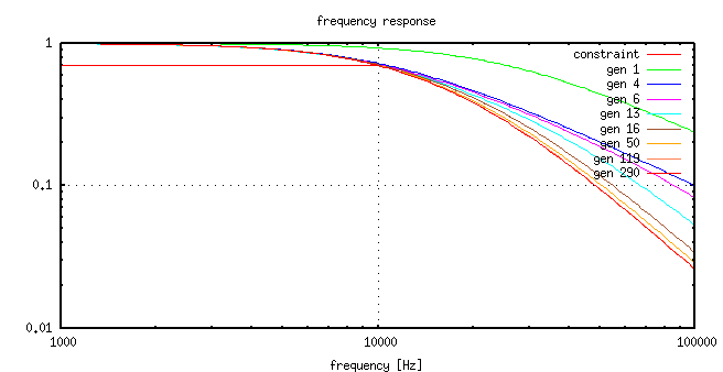
Below the cutoff frequency the signal level at the output has to be above 1/sqrt(2) = 0.707. This is the constraint for a lowpass filter. The cutoff frequency is defined inside the cost function. For every simulation point that violates that constraint I sum up a high penalty, e.g. 1 million.

Above the cutoff frequency there should be no signal. Well, no signal is not possible, but we can optimize the parameters to make the signal above the cutoff frequency as low as possible. As cost function I just sum up the amplitudes of the simulation values.

Note: As the constraint cost is much higher than the optimization cost, the optimizer will first fulfil the constraint and after that start the optimisation.

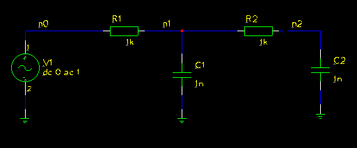
All part values have predefine value ranges. Usually nobody uses large capacitances or very small resistance values. That ranges are defined in the parameters structure.

progress of the optimization

If you have only two values to optimize you can use an XY-plot of the population parameters, too.

The following graph shows the cost after the first few parameter generations

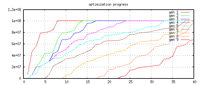
After the fifteens step, every parameter set fulfils the contraint function an the plot of the cost values rescales.

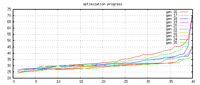
The cost graph becomes flatter and flatter. If the graph does not longer change very much, it's likely that the optimizer found a good parameter set for the problem.

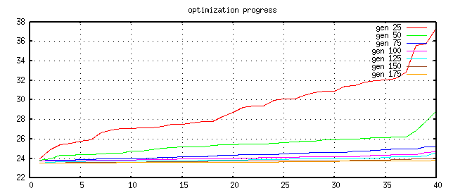
After about 200 generations the result seems to be close at the optimum point.

Iteration=200,  Best=2.353330e+01, cost_max=2.371315e+01,  cust_sum=9.443513e+02
best(1)=1.000237e+03  [1.000003e+03, 1.111371e+03]
best(2)=9.953464e+03  [9.284823e+03, 9.998692e+03]
best(3)=1.040548e-08  [9.269194e-09, 1.107771e-08]
best(4)=9.158298e-10  [8.664365e-10, 1.060045e-09]

The corresponding values to the graphs are:

gen. cost-value    R1 value      R2 value      C1 value      C2 value
-------------------------------------------------------------------------
1    5.662344e+01  2.804826e+03  5.016530e+03  2.012948e-10  7.849078e-10
4    3.201472e+01  9.894972e+03  3.881069e+03  1.368857e-09  1.505603e-10
6    3.068797e+01  5.292370e+03  4.089315e+03  2.561857e-09  3.286352e-10
13   2.823533e+01  1.245779e+03  1.496412e+03  9.375706e-09  2.347155e-09
16   2.584715e+01  2.162824e+03  9.980067e+03  5.568652e-09  5.877688e-10
50   2.432388e+01  1.043795e+03  5.612230e+03  9.591718e-09  1.509151e-09
119  2.360833e+01  1.005972e+03  9.710440e+03  1.047474e-08  9.197885e-10
290  2.352395e+01  1.000819e+03  9.997582e+03  1.021856e-08  9.290190e-10

Example 2: CMOS inverter

• The crosscurrent at the switching point should be 1mA
• The switching point should be at Vcc/2
• The maximum of the crosscurrent lies at the switching point

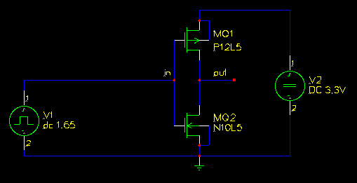
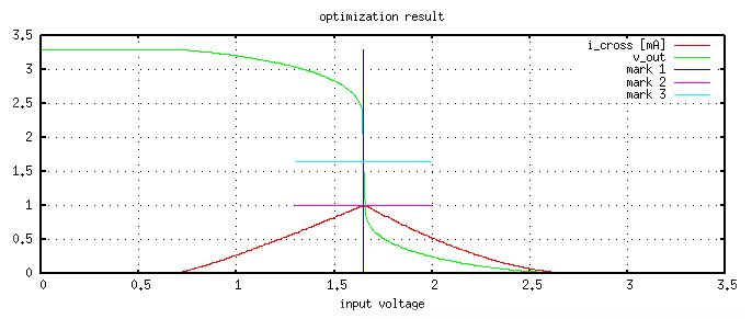
The result of the optimization looks like this:

The optimisation progress table of that run was:

gen. cost-value    M1 length     M1 width      M2 length     M2 width
-------------------------------------------------------------------------
2    3.716249e+00  1.510325e-06  7.798511e-05  2.073922e-06  4.611444e-04
2    1.408342e+00  4.322362e-06  8.861741e-05  1.917413e-06  1.569822e-04
3    3.771702e-01  8.795242e-06  2.642304e-04  2.499718e-06  3.134509e-04
7    2.084642e-01  2.452974e-06  5.018399e-05  4.700672e-06  4.917347e-04
28   1.971755e-01  2.154091e-06  5.045458e-05  1.774857e-06  1.653767e-04
88   1.617096e-01  9.720249e-06  2.863535e-04  3.053421e-06  3.982465e-04
144  1.564798e-01  3.668417e-06  9.669770e-05  1.561664e-06  1.476800e-04
199  1.082068e-01  9.836934e-06  2.305452e-04  3.946488e-06  4.306234e-04
214  1.043691e-01  6.950546e-06  1.795173e-04  3.856918e-06  4.637418e-04
232  5.164239e-02  6.356350e-06  1.613084e-04  3.870419e-06  4.622413e-04

Example 3: impedance matching

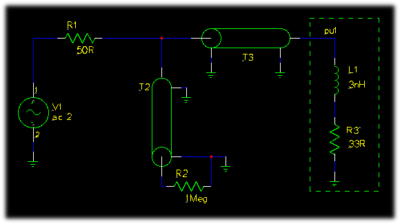
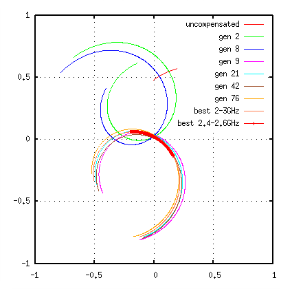
At that connection of R1, T2 and T3 the incident and reflected voltage are there. To get the reflected voltage the incident voltage has to be removed.

The reflection coefficient ist V_reflected/V_incident. As V_incident is 1V, the reflection coefficient is equal to V_reflected.

The next graph shows the reflection in the complex plain.

The optimisation progress table of that run was (some lines removed):

gen. cost-value    T2 Z0         T3 Z0         T2 TD         T3 TD
-------------------------------------------------------------------------
0    59.605        50            50            1e-12         1e-12
2    4.879770e+00  4.711152e+01  1.156916e+02  1.535854e-10  1.608469e-10
8    3.918364e+00  5.757418e+01  8.546133e+01  1.436777e-10  1.462799e-10
9    3.366191e+00  6.433881e+01  7.151574e+01  5.831321e-11  1.822875e-10
21   3.332348e+00  4.894428e+01  6.274242e+01  5.178099e-11  1.796019e-10
[...]
42   3.247336e+00  4.624785e+01  6.786233e+01  5.044231e-11  1.807375e-10
[...]
76   3.165438e+00  4.324340e+01  5.498546e+01  5.053047e-11  1.792231e-10
[...]
303  3.075487e+00  4.000000e+01  5.946972e+01  4.737848e-11  1.797402e-10

Download

Links